Gas Lift and Sensitivity Analysis

Restore production with gas lift and evaluate injection-rate sensitivity.

The fluid characteristics in the previous tutorial produced a well that could not deliver oil to a 3000 kPa system. If the separator pressure cannot be reduced, an artificial lift method such as gas lift can be evaluated.

Video tutorial coming soon

A YouTube walkthrough will be embedded here.

1. Upload the File

Select Home in the sidebar.
Select Clear All Data to start from a clean model.
Select Upload File and choose the file saved in the previous tutorial, for example model_well_tutorial_3_nodal_YYYYMMDD.

2. Add Gas Lift

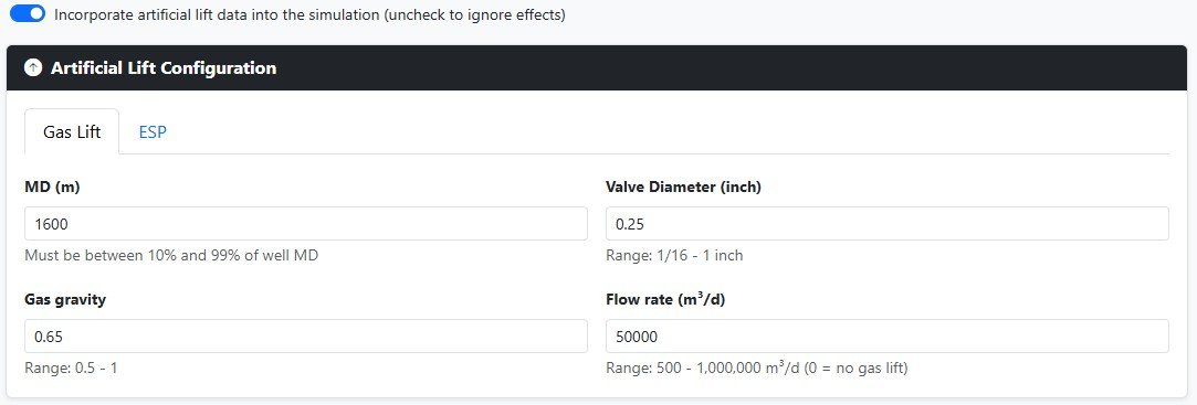
Select Art. Lift in the sidebar and check Incorporate artificial lift data into the simulation.
Select the Gas Lift tab.
Enter MD. Use 1600.
Enter Gas gravity. Use 0.65.
Enter Valve Diameter. Use 0.25.
Enter Flow rate. Use 50000.

A valve diameter of 0.25 in corresponds to a 1/4 in gas lift valve diameter. The validation messages will clear because all required checks have passed.

Gas lift inputs used to restore production.

Select Simulation in the sidebar.
Select the Nodal Analysis tab.
Select Run Nodal Analysis.

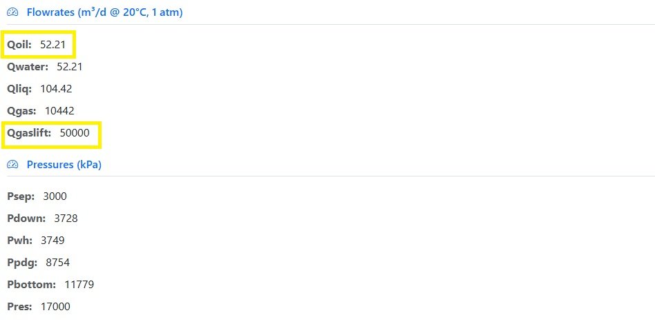
Nodal Analysis results with gas lift — Nodal Analysis results after applying gas lift. The well becomes productive.

After applying gas lift, the well becomes productive. In the previous case there was no operating point, but now the model shows an oil flow rate of approximately 52.21 m³/d.

3. Review Curve Crossing and Pressure Profile

Open the Curve Crossing plot and select Nodal at Surface.

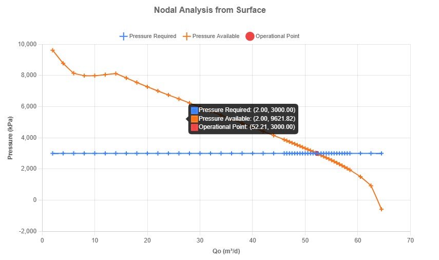
Nodal Analysis curve crossing with gas lift — Curve crossing with gas lift. The oil rate establishes the equilibrium point.

An oil flow rate of approximately 52.2 N m³/d establishes the equilibrium.

Open the Pressure Profile plot and select Pressure Profile for Well.

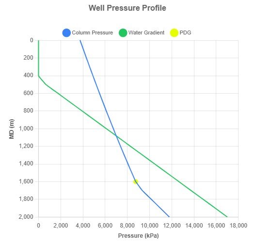
Pressure profile with gas lift. The flowing pressure gradient is reduced above the injection point.

The pressure-drop rate is lower from 1600 m to the surface because gas lift reduces the flowing pressure gradient. This is an expected and desirable effect.

4. Run Sensitivity Analysis for Gas Lift

Select Simulation in the sidebar.
Select the Sensitivity tab.
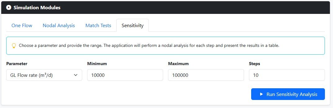
Select Parameter. Use GL Flow rate.
Enter Minimum. Use 10000.
Enter Maximum. Use 100000.
Enter Steps. Use 10, the maximum currently available.

TapirFlow offers other parameters for sensitivity analysis. The objective variables may differ from this example, but the workflow is similar.

Gas lift sensitivity analysis inputs — Sensitivity analysis inputs for gas lift flow rate.

Select Run Sensitivity Analysis.

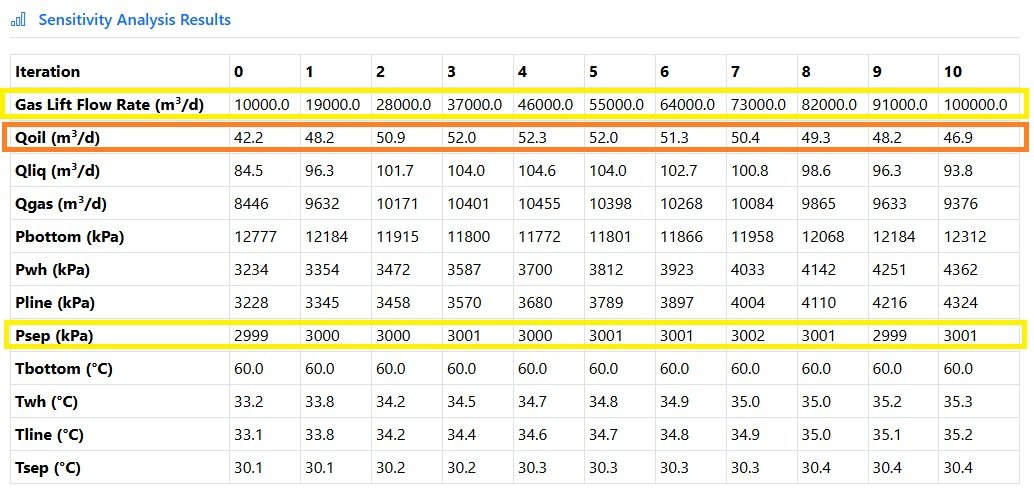
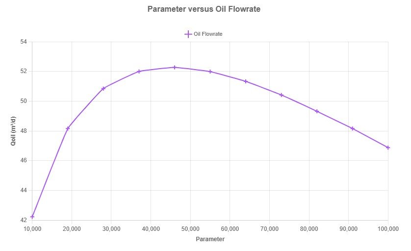
Gas lift sensitivity analysis results — Sensitivity results for gas lift injection rates from 10000 to 100000.

The gas lift flow rate ranges from 10000 to 100000 in tem divisions, as configured. All iterations converge, and Psep remains close to 3000 kPa. The oil flow rate starts to decrease from iteration 5, which indicates that excessive gas injection can reduce oil production. In this example, the optimum rate is close to 46000 m³/d.

Oil rate response to gas lift injection rate. The optimum is close to 46000 m³/d.

5. Save the Gas Lift Sensitivity Model

Select Home in the sidebar.
Enter Model Name. Use Well Tutorial-4.
Enter Model Description. Keep Tutorial to get used to TapirFlow.

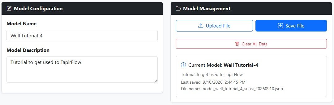
Tutorial 4 home page with gas lift sensitivity model information — Model information after the gas lift sensitivity analysis.

Select Save File. TapirFlow will save a file named model_well_tutorial_4_sensi_YYYYMMDD. Move it to your Tutorials folder.

{% endblock %}