Basic Simulation

Build a simple well model and run a One Flow simulation.

One Flow calculates the pressure drop from bottomhole to the surface for a specified flow rate and returns the pressure at the final node. In this tutorial, you will configure fluid, reservoir, and well data for a simple fictional system.

Video tutorial coming soon

A YouTube walkthrough will be embedded here.

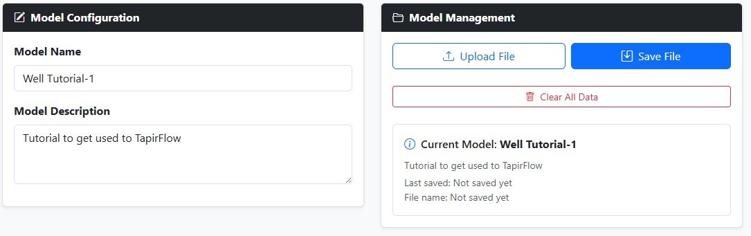
1. Home Page - Enter General Information

Select Home in the sidebar.
Select Clear All Data to start from a clean model.
Enter Model Name. Use Well Tutorial-1.
Enter Model Description. Use Tutorial to get used to TapirFlow.

TapirFlow home page with model information — Home page fields used to identify the first tutorial model.

2. Fluid Page - Enter Fluid Properties

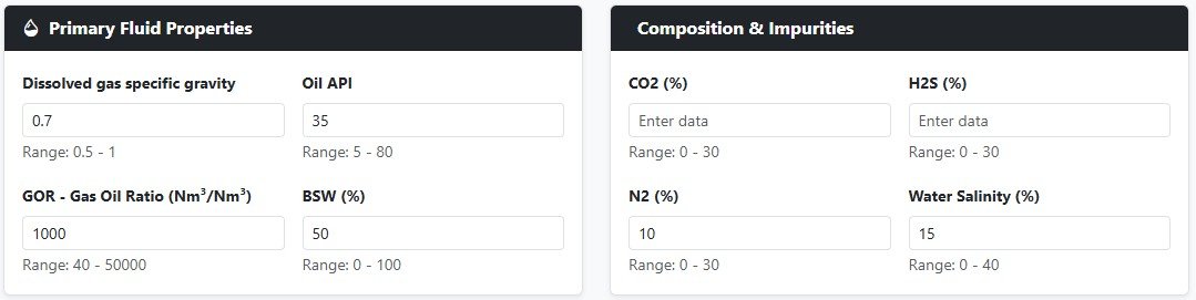
When you open the page, validation messages may appear because some required fields are empty. Enter the following values:

Select Fluid in the sidebar.
Enter Dissolved gas specific gravity. Use 0.7.
Enter Oil API. Use 35.
Enter GOR - Gas Oil Ratio. Use 1000.
Enter BSW. Use 50.
Enter N2. Use 10.
Enter Salinity. Use 15.

Fluid properties entered for the first simulation — Fluid properties used in the first One Flow simulation.

3. Reservoir Page - Enter Reservoir Properties

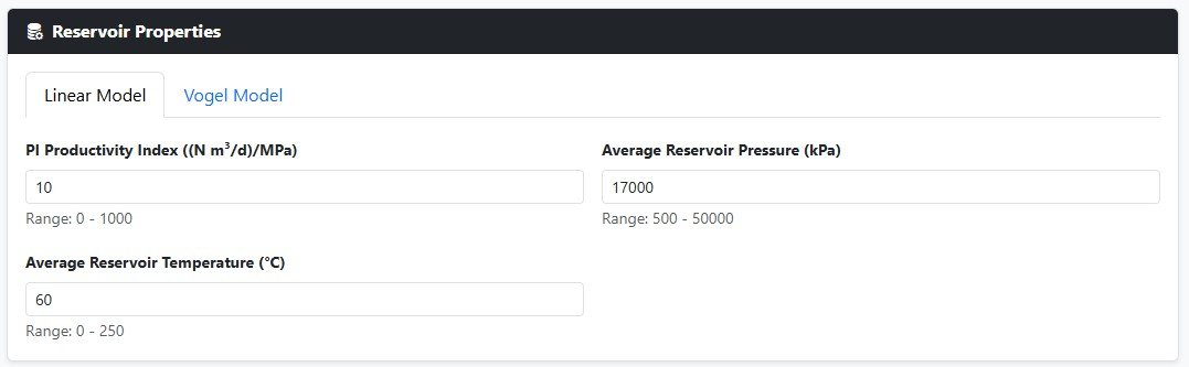
TapirFlow provides two IPR methods at this stage: Linear and Vogel. This tutorial uses the Linear model.

Select Reservoir in the sidebar.
Select the Linear Model tab.
Enter PI Productivity Index. Use 10.
Enter Average Reservoir Temperature. Use 60.
Enter Average Reservoir Pressure. Use 17000.

Reservoir Linear IPR inputs — Linear IPR inputs for the reservoir model.

SelectPlot Curve to view the Linear IPR curve.

You can also switch to the Vogel Model tab, enter the same required inputs used for the Linear Model, and enter Maximum Oil Rate as 100. Select Plot Curve again to view both IPR curves.

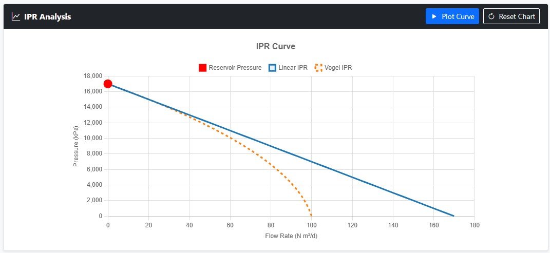
Example Vogel IPR curve generated from the reservoir inputs.

Return to the Linear Model tab and leave it active. The active tab is the model that will be used in the simulation.

4. Well Page - Enter Well Properties

Select Well in the sidebar.
Enter Rugosity. Use 0.05.
Enter Heat Coefficient. Use 30.
Under Casing Properties, enter ID. Use 150.4.
Under Casing Properties, enter Bottom hole MD. Use 2000.
Under Tubing Geometry, enter Tub ID. Use 62.
Under Tubing Geometry, enter MD. Use 1700.
Under Tubing Geometry, enter TVD. Use 1700.

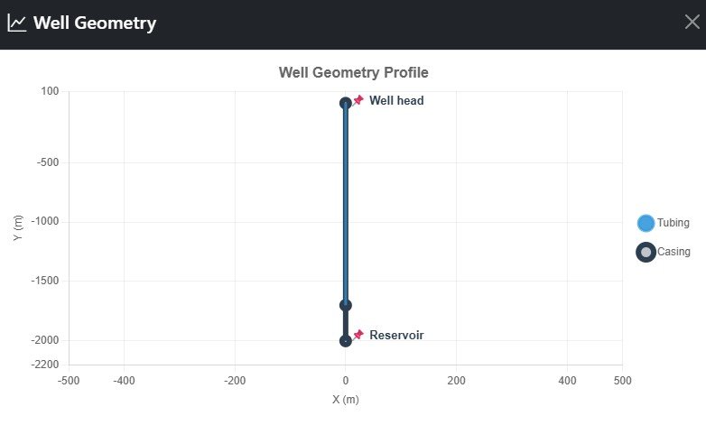
Because MD and TVD are equal, the well is vertical. The angle will be 90 degrees, measured from the horizontal line of the segment.

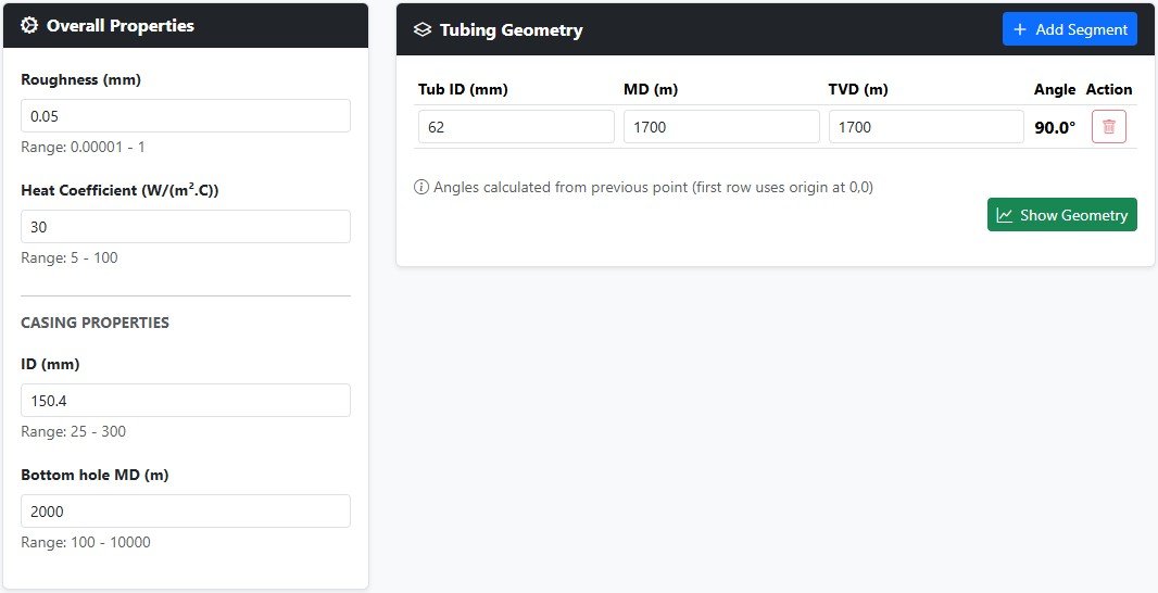
Well inputs for casing and tubing geometry — Casing and tubing geometry used for the first tutorial well.

Select Show Geometry to view the well geometry.

Discretized well geometry — Discretized geometry of the vertical well.

5. Artificial Lift and Flowline Pages

Select Art. Lift in the sidebar and verify that Incorporate artificial lift data into the simulation is unchecked.
Select Flowline in the sidebar and verify that Incorporate flowline data into the simulation is unchecked.

6. Simulation Page - Enter Simulation Information

Select Simulation in the sidebar.
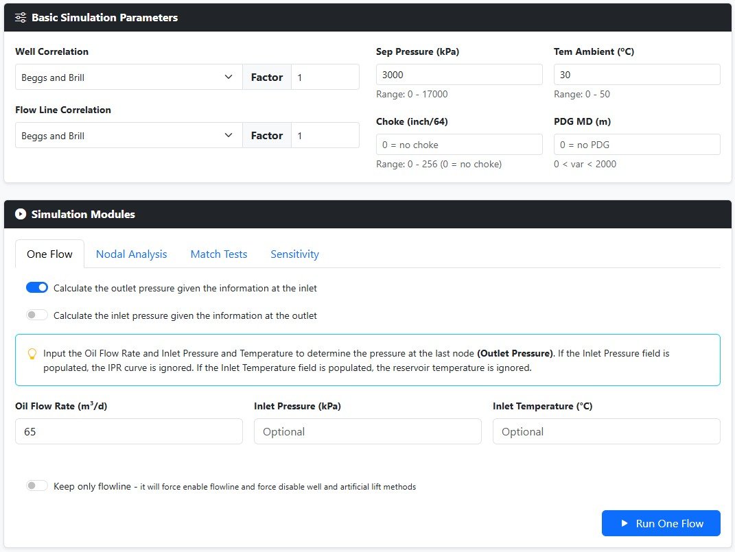
Select Well Correlation. Use Beggs and Brill, and set the pressure-drop Factor to 1.0.
Select Flow Line Correlation. Use Beggs and Brill, and set the pressure-drop Factor to 1.0.
Enter Sep Pressure. Use 3000.
Enter Tem Ambient. Use 30.
Select the One Flow tab.
Enter Oil Flow Rate. Use 65.
Leave Inlet Pressure and Inlet Temperature empty.

For a One Flow simulation, Sep Pressure is not directly used in the calculation if Calculate the outlet pressure given the information at the inlet is selected. It represents the pressure at the final node and becomes the main system constraint in other simulation types. Leaving them empty tells TapirFlow to use the IPR curve.

One Flow simulation inputs — One Flow inputs with Bottom Pressure intentionally empty.

7. Settings Page

Select Settings in the sidebar.
Verify that Discretization length is 100 for both Well and Flowline.

8. Save and Upload the Model

Saving the model is a good practice because it prevents you from entering the same data again later. Select Home, then select Save File. TapirFlow will save a file named model_well_tutorial_1_oneflow_YYYYMMDD to your downloads folder.

Create a folder named Tutorials and move the saved file into it. To test the upload workflow, return to Home, select Clear All Data, then select Upload File and choose the saved file.

9. Run the One Flow Simulation

Select Simulation in the sidebar.
Select the One Flow tab.
Select Run One Flow.

If everything is configured correctly, the simulation results will appear immediately below in the Stored Simulations table.

Click on View Results to switch to the Results page.

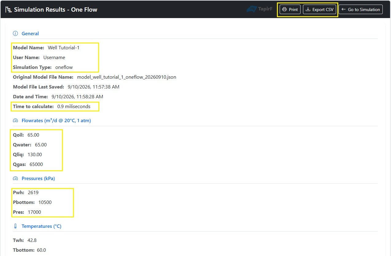
One Flow simulation results — One Flow results showing general information, flow rates, and pressures.

In the results page, review the following sections:

General: model name, user name, simulation type, and calculation time.
Flowrates: Qoil, Qwater, Qliq, and Qgas.
Pressures: Pwh at the wellhead, Pbottom at the bottomhole, and Pres at the reservoir.

10. Review Result Plots

At the bottom of the Simulation Results page, select Plots to view the available plots.

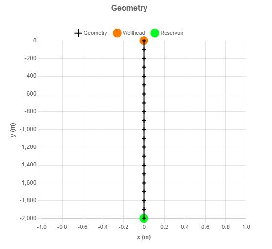
Geometry

The Geometry plot shows the discretized geometry.

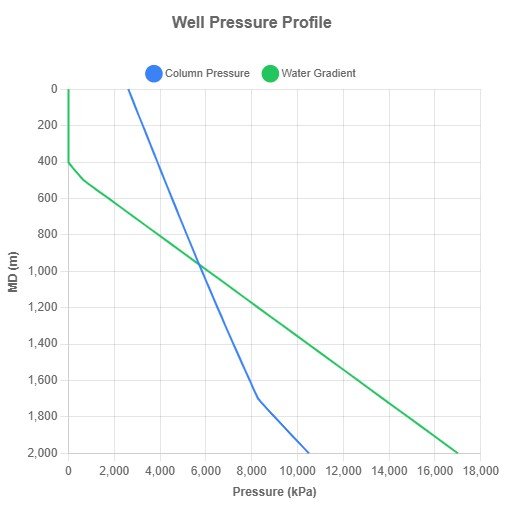
Pressure Profile for Well

The Pressure Profile for Well plot also provides an estimate of the static level using the water gradient. In this case, the static level is expected to be between 500 m and 400 m.

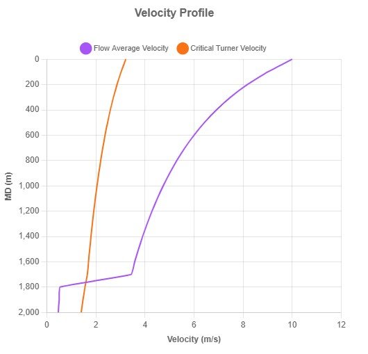
Pressure profile for the well and estimated static level from the water gradient.

Velocity Profile for Well

The Velocity Profile for Well plot provides an estimate of the Turner critical velocity for liquid loading.

Velocity profile with Turner critical velocity reference.

Final discussion: In this example, P_wh is approximately 2619 kPa. As an exercise, find a Well Correlation Factor that better matches the target wellhead pressure of 3000 kPa. The factor should be approximately 0.946 which brings P_wh to very close to the target.